

by Dr. Matthew Templeton, AAVSO
(Copyright 2003, AAVSO. All rights reserved.)
The full version of this paper appears in the Journal of the AAVSO, volume 32, number 1, page 41.
In this short paper, I'll give a very brief overview of time series analysis, broadly discussing how time-series analysis is performed on astronomical data, and what we can hope to get from it. I'll also suggest different kinds of analysis for different kinds of objects, and then suggest some resources that you might find useful in your own work.
It might help to give a formal definition of what time-series analysis is before we start discussing it.
I define time-series analysis as the application of mathematical and statistical tests to any set of time-varying data, both to quantify the variation itself, and to use that variation to learn something about the behavior of the system.
Ultimately, the goals of time-series analysis are to gain some physical understanding of the system under observation: what makes the system time variable, what makes this system similar to or different than other systems with similar variability, and so on. The other goal is to perhaps be able to predict future behavior; if not an exact prediction, then at least some quantification of the limits of the system.
One thing it's important to realize is that time-series analysis isn't a field unique to astronomy. It has relevance to lots of different areas, from radio and telecommunications to forecasting (from financial to weather!), to various engineering disciplines. Time-series analysis is a field that many people have put a lot of work into over the past several decades, and there are always new ideas and new methods being introduced. So it is a very rich field of research.
Here is a roadmap of what I want to talk about today.
I'm going to start with a discussion of statistics, both to introduce those of you who are new to time-series analysis and to statistics, and to show the relevance of statistics to time-series analysis.
Then I'll cover three areas of time-series analysis, namely Fourier analysis and Fourier transforms, wavelet analysis, and autocorrelation, all of which are well-suited to working with AAVSO data.
And then finally, I'll list some resources that you can use to begin your own studies.
The two concepts I want to discuss regarding statistics are the mean, and the variance or the standard deviation.
The concept of mean value of a set of data is very straightforward one. If you take the sum of a given set of data values, and then divide the sum by the number of values you added together, you obtain the arithmetic mean, or the average. (For the sake of simplicity, I'll be calling this the mean, though a statistician would argue that the true mean is actually an expectation value -- the average you theoretically expect for a given statistical test.)
For example, say you have a set of ten measurements of anything, be they magnitudes, shoe sizes, or batting averages. If you sum those ten measurements together, and then divide the sum by ten, you obtain a mean value about which these measurements are distributed. Simple enough, but mean values are very important to time-series, as I'll discuss in a moment.
The concepts of variance and standard deviation are also straight forward, especially since they follow naturally from defining the mean. The variance is defined as the sum of the squared differences between each measurement and the mean, given by

and the standard deviation is the square root of the variance. Basically, the standard deviation is a measure of how far, on average, the data points lie from the mean value. If you can quantify how much the data vary about the mean value, and if you know (or suspect) that the mean value is close to the "correct" value, then the standard deviation allows you to quantify how "good" the data are - the smaller the standard deviation, the more accurate most of the data points are.
Many of you have probably heard of the term "sigma" used in this context, and sigma is just another term for the standard deviation. However, sigma is usually used in terms of how good a particular result is, like "these are one-sigma error bars" or "this is a ten-sigma result!!" I've created a visual to show what the standard deviation and sigma mean in terms of data quality and consistency.
Here, I've generated a 5000-point, synthetic data set consisting of averaged random numbers: each data point is an average of 1000 random numbers between 0 and 10. The result is the data on the left. I then asked how are those values distributed about the mean? The result is the histogram shown on the right. As one might expect, the true, statistical mean is precisely 5, and the measured arithmetic mean is very near 5 (here, it is about 4.994). But we're also interested in how much spread there is about the mean. I placed one and three sigma error bars on the histogram. One sigma means that 68% of the data lie within one sigma of the mean, and three sigma means that 99.7% of the data lie within three sigma of the mean, a very good (but not certain) probability.
So what does this mean?
This lets us quantify how good our measurements are. Suppose instead of taking random numbers, we were looking at observed magnitude of a constant star. Suppose you were told that the mean magnitude was 5, with a one sigma error bar of 0.5 magnitudes (as above). You'd then know that "most" (68%) of measurements place the star between 5.5 and 4.5 magnitudes. But if the three sigma error was 0.5, then you'd know that nearly all (99.7%) of the measurements lie between 4.5 and 5.5. If the error bars were 0.05 or 0.005, then you'd be that much more certain of your measurements.
Now, what I discussed was perfectly acceptable for talking about measurements of a static process with normally distributed errors. But that isn't the case with variable stars!
For one, the star may be undergoing brightness variations which cause the mean value to vary. If the mean varies over short timescales, then those variations might average out over time, but what if brightness variations occur over centuries or millenia? What if there are trends in the data, like in a nova or supernova fading? What is the mean value then? Does it even make physical sense to talk about a mean value?
Then there's the variance. With variable star data, it is acceptable to talk about the variance just as I described above. But you have to realize that the variance will then be a combination of many things, not just the intrinsic scatter in the measurements. You have contributions from systematic errors, such as different observers using different charts, or maybe having different optical or color sensitivities. And then of course, you have variations about the mean due to the star's varying brightness!
Sometimes this difference is important, particularly when we want to talk about the signal to noise ratio of the data. Signal to noise generally refers to the amount of signal compared to the amount of intrinsic scatter, so including the real variations isn't appropriate. However, at other times, this measurement of variance is key, particularly if you're using a statistical method like the ANOVA test to find periods that minimize the total variance in the data.
So to summarize what I talked about here, you should basically have two things in mind regarding statistics and "data quality."
First, realize that you will always have some amount of error in your data, regardless of how big your telescope is, how bright or faint the star, and how long your integrations. Even the very fact that light is composed of individual photons introduces an intrinsic noise to the system.
Second, also realize that some systematic things contribute to the data variance, and you must take this into account when performing a statistical (and time-series) analysis. Be aware of this before you jump in and start "crunching numbers"
Now that we have statistics out of the way, we're moving on to methods of time-series analysis. As I said, I'll be covering three types of analysis useful for AAVSO data.
First, I'll cover Fourier methods, in which one attempts to reconstruct a signal with a series of trigonometric functions. They are one of the oldest forms of time-series analysis (barring perhaps brute-force period-folding), and are also quite flexible.
Then I'll discuss a relatively new form of analysis called wavelet analysis, which analyzes the data in small pieces, and tries to fit short periodic functions (or wavelets) to the observed variations. Although it is a form of Fourier analysis, it is distinct in that it was designed from first principles to track the evolution of the variability over time. Again, this is useful for objects whose behavior changes with time.
Finally, I'll talk briefly about autocorrelation, which is a more statistical approach than a trigonometric one. Instead of fitting a dataset with trigonometric functions, you compare points in the dataset to other points at fixed time intervals or "lags" to see how different they are from one another. As I'll show, this has some utility for analyzing stars that may have some intrinsic "period" but are far from regular pulsators.
I'll spoil the punchline of the whole talk by saying ahead of time that you should always make an assessment of what you want to study and how you should go about it, and that you should try to use the right tool for the right job. Some methods may be interchangeable, like wavelet and Fourier analysis, but depending upon the amount of data and your desired goals, there may be an optimal choice of analysis techniques.
Fourier analysis attempts to represent a set of data with a series of sines and cosines with different periods, amplitudes, and phases. In so doing, you can estimate the periods of variability by finding out which of these sines is strongest.
This representation is done by a mathematical process called a transform, which is exactly what occurs - the data measurements in the time domain are transformed into the period or frequency domain.
This transformation of variables is done with an equation called the Fourier transform,
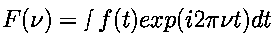
Real data, given by the f(t) values, is not an analytic function, which means that the integral above must be performed numerically. For each period or frequency you want to test (given here by the Greek letter nu), you perform the integration above: multiply each measurement in time by the complex exponential function shown (which Euler showed is a complex sum of a sine and cosine) and the time difference between each point, and then sum over all of the measurements. Then you move on to the next period you want to test, and perform the integration again, and again, and again.
There are probably dozens if not hundreds of different numerical algorithms and computational methods to actually perform the Fourier transform, but all of them share this idea.
Now that we know in principle how to perform a Fourier transform, the question becomes how do we select the periods that we want to test? We don't want to select periods at random, and we don't want to do too many or too few tests. The answer is that you choose the periods you want to test based upon the data set itself. It is your data that place limits on both the resolution of your period search (how far apart the test periods should be spaced), and on the longest and shortest periods you're allowed to test.
Ultimately, the thing to remember is that the shorter the time span of data you have, the worse will be the resolution and range of your transform.
As an example, suppose you have a data set spanning 5000 days, with a sampling rate of 10 data points per day (separated by 0.1 days) What are the optimal maximum and minimum periods and period resolution or sampling for your data set?
The optimal sampling of periods (or frequencies) are defined by the parameters of your data, particularly by the rate at which you make observations - called the sampling rate, and the time span of your data.
The sampling rate defines a very important quantity, called the Nyquist frequency. The Nyquist frequency is the frequency of a sine wave exactly half that of your sampling frequency. If you record a sine wave having the Nyquist frequency, then you obtain two samples per cycle, and can in principle sample the wave at its peak and trough. The Nyquist frequency places an upper limit on the frequencies you can search for in a given data set with some sampling rate.
So since our sampling frequency is ten times per day, our Nyquist frequency or maximum test frequency is half that: 5 times per day, corresponding to a minimum test period of 0.2 days. (In a moment, I'll tell you why we can cheat and get around the Nyquist frequency sometimes, but for now, take this as a given).
The minimum frequency (or maximum period) is given by the span of the data itself. In principle, the maximum period you could test for is 5000 days - you could see the data pass through one peak and one trough. However, this assumes that you know in advance that the data is periodic. A more rigorous constraint is that your data should contain at least two cycles. So in this case, the maximum period you could test for is half of the time span, or 2500 days.
Last is the frequency or period sampling. According to the sampling theorem any set of data containing a signal with a frequency lower than the Nyquist frequency can be fully described by a set of frequencies given by n/ND, where N is the number of points, D is the spacing of the data points, and n is a number between -N/2 and N/2. The negative frequencies (n = -N/2 to -1) are equivalent to positive frequencies (N - n), so the transform is usually computed for frequencies with n between 0 and N-1 instead.
This is the most efficient sampling required to fully extract all information from the signal. In practice, one can oversample the frequency/period spacing to any degree that your computational facilities permit and for all but the largest datasets, it is now easy to oversample by a factor of two, four, or more to improve the smoothness of the output transform. However, in order to fully sample the Fourier transform, the spacing of periods must be at least this fine.
The frequency sampling is quite important for two reasons. First is one of efficiency: you want to obtain the most information you can from your data, but you don't want to drastically oversample your Fourier transform and waste lots of computer time. The second is that it gives you some clue as to how precisely you can determine the period. This slide shows an example of the practical limits on precision set by the time span of your data.
Here are two Fourier transforms of data on the Mira star R CVn. According to the GCVS, the period is about 329 days, corresponding to a frequency of about 3 one thousandths of a cycle per day. The transform on the left used data spanning only the last seven or so years, while the data on the right spans over 97 years. Both transforms recover the dominant peak at nearly the same frequency, but the transform with more data defines the period much more precisely. So the longer the span of data you have, the better your precision.
One last point on sampling. Remember I said that the Nyquist frequency places an upper bound on the test frequencies, corresponding to a lower bound on the periods you can test for. However, you can, in some cases, test for frequencies higher (often much higher) than the Nyquist frequency. You can do this so long as the data points are not evenly sampled, and so long as the points adequately cover the light curve in phase over the length of the data set. This "additional information" comes at the cost of a major headache, namely aliasing. Aliasing occurs where the Fourier transform shows a power peak at the correct frequency, but also shows statistically significant peaks at different frequencies. The location and spacing of these alias peaks is a function of the data sampling. For example, data with daily gaps will have aliases of one cycle per day, and data with annual gaps will have aliases of one cycle per year.
For example, the slide shows a Fourier transform of a delta Scuti star observed by the MACHO Project. MACHO data is sampled on average (but not exactly) once per day during the observing seasons for the Galactic bulge and the Magellanic clouds. As a result, the Fourier transform is able to pick up a pulsation frequency (5.5/day) much higher than the sampling frequency (1/day), but there are alias peaks surrounding the main peak separated by one cycle per day. This is common in real data analysis, particularly when dealing with data of short period stars like RR Lyrae, delta Scutis and white dwarfs. The solution is to try subtracting a sinusoid having the frequency, amplitude and phase of the strongest Fourier peak from the data, a process called prewhitening. Doing so should make the strongest peak and the alias frequencies disappear when you transform the prewhitened data.
Now that I've described what Fourier transforms are and what considerations have to be made when using them, I wanted to quickly mention some different classes of algorithms that you may come across. There are many different individual algorithms used for time-series analysis, and each usually has a different application.
First is the classical discrete Fourier transform (DFT) which is a discretized version of the Fourier transform integral I showed several slides ago. It was originally intended for regularly sampled data, and was developed as early as the 18th century.
The fast Fourier transform (FFT) is what its title implies -- a fast and efficient method for performing a Fourier transform. It takes advantage of some peculiarities of transforms and the Sampling theorem to extract all of the information a data set can yield with far less computational time than the discrete transform. Since it requires regularly sampled data, it isn't ideally suited for many astronomical applications, especially AAVSO data. However, for applications like "real-time" signal processing and analysis of very large data sets (e.g. billions of data points), there's really no other choice.
Though the method may have first been derived by Gauss in the early 19th century, it is commonly referred to as the Cooley-Tukey algorithm, after two computational scientists of the 1960s. It is also occasionally referred to as the Danielson-Lanczos algorithm.
The date compensated discrete Fourier transform (DCDFT) is an implementation of a discrete transform first derived by Ferraz-Mello in 1981. This algorithm was modified and implemented as the CLEANEst algorithm by Grant Foster, and is available as part of the AAVSO's "TS" analysis package. As the name suggests, it takes the time of observation into account, meaning that the data no longer has to be regularly sampled. It works quite well with AAVSO data, and should have no trouble with most of your data analysis needs.
Another algorithm you might come across is the Lomb-Scargle periodogram, also useful for unevenly-sampled data, and in very common use. The method was derived by Lomb in 1975, with improvements by Scargle in the 1980s. Although the Lomb-Scargle periodogram decomposes the data into a series of sine and cosine functions, it is similar to least-squares methods, and thus also uses statistical analysis. The periodogram is often used as a test of the significance of periods in data, though the DCDFT/CLEANest algorithms can also produce similar statistics.
So now that we have all of that information under our belts, what do we do with it? Well, you can use Fourier analysis techniques to work with all kinds of data, and there are ways to analyze nearly every kind of signal you may expect to encounter, using Fourier techniques or variants thereof.
Some things that I've used Fourier analysis to study in my own research include:
Multiperiodic data: some stars (especially delta Scuti stars, white dwarfs, and the Sun) pulsate in multiple pulsation modes simultaneously, and Fourier transforms provide an efficient way to uncover multiperiodic signals. Typically what one would do is obtain a Fourier spectrum of the raw data, find the highest peak, then either subtract it from the data and transform it again, or compute another transform assuming that the first peak is real and search for the next peak. You then iterate this until you can't see any more periods in the data. You may have to repeat this dozens of times depending on the star you're observing.
Another application is the study of "red noise" - excess power above the noise level, often seen at low frequencies in the Fourier transform. It is due to long-term, incoherent variations in the system being observed. This sort of "temporal noise" is very common in accreting stars (particularly x-ray binaries) and the slope of the spectrum may provide some information on the accretion dynamics.
You can also study period and amplitude evolution. Changing periods and amplitudes will often show up as additional peaks in the Fourier spectrum surrounding the main peak. Analyzing these peaks can tell you how the signal varies with time.
And finally, one can uncover the "shapes" of lightcurves by using the Fourier transform to obtain the Fourier harmonics in a signal. I'll show an example of that in the next slide.
Another concept associated with Fourier is that of the Fourier series. Basically, a Fourier series is an attempt to represent any kind of periodic signal with an infinite series of sine or cosine waves. By periodic, I mean something like a sawtooth wave, which may have a well-defined period, but which is definitely non-sinusoidal. In this case, you can represent a sawtooth wave with an infinite number of sine waves, beginning with one sine wave having the same period as the sawtooth wave, then the next with half the period, then the next with one third the period, then the next with one fourth the period, and so on.
This idea has real utility when talking about some pulsating variable stars, notably Cepheids, RR Lyrae, and high amplitude delta Scuti and SX Phoenicis stars. These stars are by and large strictly periodic, but have markedly non-sinusoidal light curves. What has been found over the past several decades is that the shape of the lightcurve is often correlated with other physical properties, like the star's period. In fact, there's a significant change in the shapes of Cepheid light curves at periods around 10 days.
One way to measure the light curve shape is to perform repeated Fourier analyses of a given light curve, and extract the properties of the "sine waves" in this infinite series. Here, I tried this on the delta Cepheid star AW Persei, using data from Wayne Lowder. On the left is a Fourier transform showing the main period at 6.46 days, and then the "harmonics" at one-half and one-third the period. On the right, I then show the resulting "reconstructed" light curve overlaid with a small portion of the observations, and the observations fit quite well. So it's possible to use Fourier analysis to recover light curve shapes when the light curve isn't necessarily well-sampled in time.
Now I want to talk about another, very useful method of time-series analysis, called wavelet analysis. Wavelet analysis is similar in spirit to Fourier methods in that it attempts to fit periodic functions (wavelets) to a set of data. What sets wavelets apart, however, is that wavelets were designed from first principles to study how the signal changes over time. Where Fourier methods usually involve analyzing the entire signal at once, wavelet analysis assumes that the signals may be of finite duration. So it is designed to study the spectrum of variability as a function of time.
This is an extremely useful technique for looking at stars whose periods change over measurable timescales.
In fact, many kinds of stars show either variations in period, or show no fixed period at all, instead showing transient periodicities or quasiperiodicities.
Some examples include:
The long period stars. Many of these stars including Miras show some variation in period over long timescales. Still others, like the semi-regulars and RV tauri stars show transient periods, or perhaps complex interactions between multiple periods that make the signals look very complex.
Other stars may undergo fundamental changes in their pulsation behavior on very short timescales. For example, stars may undergo "mode switches". This is where a star may pulsate at one period for a time, then begin pulsating in another period later on. An example of this is Z Aurigae, which I'll show in a moment. Another example might be a star undergoing an abrupt evolutionary change, like a shell flash in the interior. T Ursae Minoris is an excellent example of this, where we have seen the period decline by several tens of days over the past few decades.
Finally, some stars simply have transient periodicities. Examples are the CVs that exhibit transient superhumps during outburst. Wavelets could be used to pick out the period of the superhumps, and also when they started and stopped.
For the AAVSO data, Grant Foster designed and wrote a very useful form of the wavelet transform, called the Weighted Wavelet Z-Transform, or WWZ. This has been available for several years via the AAVSO website, and is very well-suited for analyzing data.
What the code does is to fit a sinusoidal wavelet to the data, but as it does so, it weights the points by applying a sliding window to the data: points near the center of the window have the heaviest weights in the fit, those near the edges have much less weight. This window is gradually moved along the data, giving us a representation of the spectral content of the signal at times corresponding to the center of that window.
When analyzing AAVSO, there are a few things to keep in mind. For one, ideal data should have a reasonably long time span, preferably much longer than the expected periods themselves. For example, if you're interested in a mira star with a period around 300 days, it would be best to have a set of data which is many times longer than that (perhaps 20 times longer) to reliably search for period changes.
Another thing to note is that WWZ allows you to select the width of the sliding window, giving you some flexibility over the sorts of timescales you wish to investigate for period changes. There are tradeoffs when making this window narrower or wider. Recall from the discussion about Fourier analysis that the span of the data has bearing on the period range and resolution. Since the data window acts to change the span of the data, making the window narrower effectively reduces the span of the data, making the period resolution worse. But by doing so, you can study period changes over very short timescales. Likewise, if you widen the window to improve the period resolution, you worsen the time resolution of the transform, making it difficult to detect short term variations.
Here we see an example of this with Z Aurigae. Z Aur is a semiregular star that is believed to undergo mode switches. The star can pulsate with periods of 110 and 137 days, and has switched between the two a few times over the past century. In the top panel, I've chosen a narrow window width, which brings out the time-varying nature of the spectrum. You can see clearly that in the early part of the data set, the period is about 110 days. This then fades, and the other pulsation period at 137 days becomes dominant. This also fades, then returns briefly before switching abruptly back to the period at 110 days. The only problem is that the periods themselves are not well-resolved, and it is impossible to define them more precisely than to within 5 or 10 days.
On the bottom panel, I chose a much wider window. This has improved the period resolution, but has nearly smoothed out all of the time variation. It also causes a problem where the strength of the signal is much lower, since it is an average of times when the period is present and when it isn't. In fact, the signal at 137 days is nearly invisible.
So when you use WWZ on your data, be aware that both the data, and your selection of analysis parameters will have some effect on the results. Apply the analysis methods wisely.
Now I want to move on from Fourier methods and conclude by talking briefly about more statistical methods of time series analysis. Earlier I emphasized that you had to distinguish between the statistical variations due to noise within the data, and those due to variations within the signal from the star itself. With statistical methods, what you are interested in are the variations due to the star. Two of the types of analysis you may be familiar with are autocorrelation analysis, and Analysis of Variance or ANOVA.
The idea behind autocorrelation is rather simple. Autocorrelation seeks to compare points in the lightcurve to other points separated by some lag time, tau. You form the autocorrelation parameter based upon whether points separated by tau are very similar, very different, or largely uncorrelated. I'll talk more about this method in a moment.
Another type of analysis is the ANOVA test. Here, the variance of the signal is the important thing. In the ANOVA procedure, you bin and fold the data with a series of test periods, and then measure the variance of the data points within each bin. If you find a minimum value of the variance at some folding period, then it is likely that the star has a real period at or near that folding period. This is the time-series algorithm that is contained within the VSTAR program
of the AAVSO’s Hands-On Astrophysics kit, so you may be familiar with it already. (Note: Since the time of publication of this article, the HOA version of the VSTAR program has been replaced with an entirely new and upgraded version which you can download from here: vstar-overview).
Unlike Fourier-based methods, instead of asking whether the light curve can be represented by periodic functions, autocorrelation asks what does the light curve look like at times separated by some interval or period tau? What autocorrelation does is take each data point, measured at time t, and then compare the value of that data point to another at time t+tau. If you perform this test for all data points, then you can average the differences together and see whether most point separated by tau are similar or different. If they're very similar, there will be a peak in the autocorrelation function at tau. If they're very different, there will be a trough. We would expect points separated by tau to be very similar if the data contained some variability with period tau, so the autocorrelation function will have peaks corresponding to periods of variability in the data.
This can be a very powerful method for stars with irregular light curves. This includes stars which are almost periodic, like some of the semiregular and RV Tauri stars, to those which may have transient periods or may have a "characteristic period" but which have generally irregular light curves. However, it isn't just mean for irregular variables. You can also use it for strictly variable stars of all types. The only difference then is whether other methods like Fourier analysis might give you more information than the autocorrelation function.
The only case where autocorrelation doesn't work so well is in stars which have multiple, simultaneous periods present in the data because the different periods interfere with one another in the autocorrelation spectrum. Fourier methods are far more straightforward in this case.
Here's one example of autocorrelation in action: R Scuti is a well-observed RV Tauri star with a "period" of about 140 days. The bottom panel shows the lightcurve of R Scuti over 2000 days. While there may be a "period" in the data, the lightcurve is far from regular. There is substantial amplitude variability, and for some cycles, the variability barely appears -- for example, note the data around JD 2448700.
By comparing the light curve at times separated by some time-difference, tau, you determine whether these points are in general correlated or not. According to the autocorrelation function, the presence of a correlation peak at about 140 days is very clear, and unambiguous. You can also see that integer multiples of this period (280 days, 420 days, and so on) are also correlated, suggesting that the 140 day period is a phased period, even though the amplitude is highly variable. However, the declining value of the correlation function peaks shows that the strength of the correlation decays over time, perhaps indicating that the pulsations decay or lose their phase coherence over time.
So I'll finish up by giving just a quick summary of what I hope you've gotten from this talk.
The main points are: one, that many different time-series analysis methods exist. The talk I gave was by no means comprehensive, though hopefully the methods I chose should be general enough to suit most of your needs. As with everything, do a little research on your own to see whether other methods or newer methods might be useful for you.
Two, choose your data analysis method carefully, and use something that's well-suited for your data. Again, do a little research ahead of time to see what might work best, and this might save you some time and trouble later on.
Finally, be aware of the limits and strengths of your data, or of any data you use. For example, visual data might not be suitable for detecting extremely low amplitude variations, but would be excellent for projects which require very long spans of data.
The following webpages have programs and additional useful information on time-series analysis, and I encourage you to visit all of them.
First, the AAVSO has the TS and WWZ computer packages for data analysis available and ready for download here.
Another excellent package is the PERIOD04 software developed by the Delta Scuti Network group at Vienna. It's very useful for Fourier analysis, and is available for both MS Windows and GNU-Linux systems, and apparently has at least a beta version available for MacOS X/Darwin systems.
The Penn State University Astronomy Department has published a substantial list of sites available from this site.
And finally, John Percy of the University of Toronto also has a web page devoted to his Astrolab package, including a page on autocorrelation.
Addendum
Since the time for my talk was limited, I couldn't cover everything, and would like to suggest a few additional resources you may wish to investigate on your own.
Nonlinear time-series
Nonlinear time-series is a relatively new and promising field of research. The premise of nonlinear time-series is that stars (or any variable physical process) may exhibit some level of chaotic behavior. Nonlinear time-series attempts to use the techniques of chaos analysis to gain physical insight into systems which cannot be analyzed by traditional time-series methods.
I recommend perusing the TISEAN website at the Max Planck Institute at Dresden. Although it is highly technical, the preprints listed on the front page are worth reading if you are interested in this type of analysis.
You might also be interested in the following paper by Buchler, Kollath, Serre, and Mattei on R Scuti.
Fourier Transforms in general
Fourier Transforms have been written about at great length for well over 50 years, and so the literature on them is very rich and varied. Beyond the links to papers I gave in Slide 15, you might find that the Numerical Recipes books by Press et al might provide some useful insight.
Statistical methods
Schwartzberg-Czerny wrote a comprehensive paper on the ANOVA method of performing time-series analysis.
A related method called phase dispersion minimization or PDM was developed by R. Stellingwerf.